Da SIMS: A KUKA youBot Simulation
*Patrick Star voice* iBot, youBot, he-she-meBot

Overview:
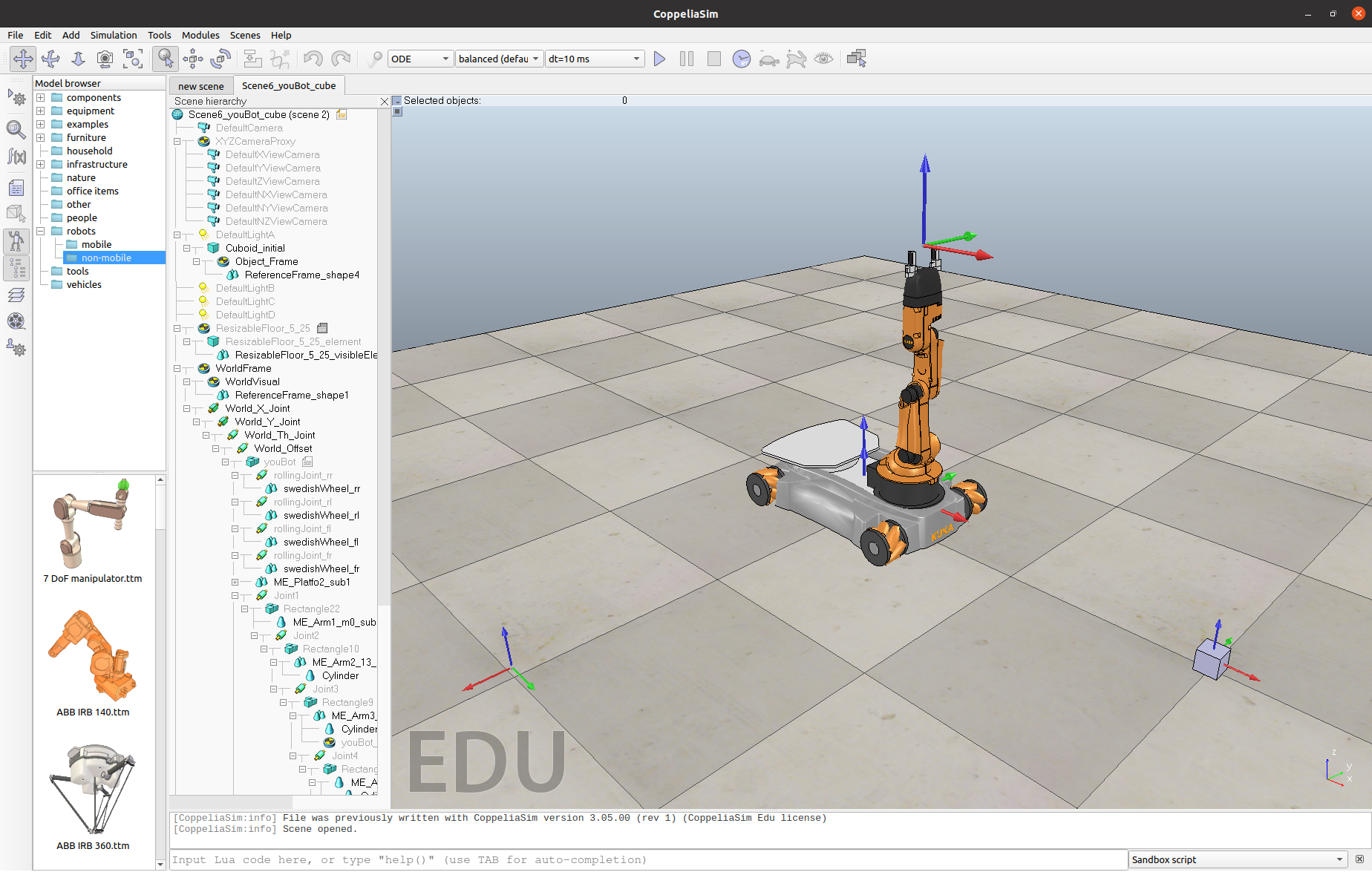
The final project for Robotic Manipulation that utilizes Python and the ModernRobotics (mr) library to manipulate a Kuka YouBot (simulated in CoppeliaSim) that picks up a block from one location and places it in another.
This simulation was repeated three times, each with a different combination of initial conditions and controllers.
More information on the project requirements and the KUKA youBot can be found here.
Components:
The deliverables of this project are as follows:
* README file (.md/pdf) to summarize findings (view)
* CODE directory containing the following:
1. TrajectoryGenerator.py
2. NextState.py
3. FeedbackControl.py
4. Mane.py*
* RESULTS directory** containing the following:
1. A brief background info README file noting the controller's type and feedback gains
2. The robot data .csv file used to run the simulation
3. A video of the simulation in action
4. The corresponding X_err .csv file
5. A plot of the X_err output over time (all 6 elements)
6. A log file showing the program being called with the input*
**The results are organized as BEST, OVERSHOOT, and NEW_TASK
*The above deliverables can be achieved by running the Mane.py script in a code editor (such as VSCode by clicking the green run button in the top right corner).
The above mentioned Python files require the following libraries:
* modern_robotics
* numpy
* logging
* matplotlib
* mrcapstone (custom made library containing the 3 milestone functions)
Please ensure that these libraries are installed before running Mane.py.
Ps: I can (mostly) spell don't worry
Instructions:
This code can be run in any code editor. All variables required are built into the code and can be edited within the .py files.
Individual calls for each function can also be found in the respective function's docstring.
Please remember to import the function before calling it!
Background:
TrajectoryGenerator.py:
The CartesianTrajectory functinon from modern_robotics was used to calculate the reference trajectory for end-effector frame {e} consisting of 8 concatenated trajectory segments which all begin and end at rest. It computes a trajectory as a list of N SE(3) matrices and then saves the eight-segment reference trajectory as a csv file.
An example call: TrajectoryGenerator(T_sei, T_sci, T_scf, T_ceg, T_ces, k)
Where its inputs are:
* end-effector initial config (T_sei)
* cube's initial config (T_sci)
* cube's desired configuration (T_scf)
* end-effector's config relative to cube @ grasp (T_ceg)
* end-effector's standoff config @ not-grasp (T_ces)
* number of trajectory reference configs per 0.01 sec (k)
k = int >= 1
and its outputs are:
* representation of N end-effector configs (each representing T_se)
* csv file of eight-segment reference trajectory
and the frames used are:
* {e}: end effector
* {c}: cube
* {s}: space
This script can be tested independently with CoppeliaSim scene 8.
NextState.py:
This script computes the new configurations of the arms and wheels and outputs the results as a csv file based on a simple
first-order Euler-step.
* F = Hcross(0) = pseudo-inverse of H(0)
* new = old + (speeds * Δt) ≤--because of Euler step
An example call: NextState(config, speeds, t_step, w_max)
Where its inputs are:
* config - 12-vector representing the current configuration of the robot
3 @ chassis, 5 @ arm, 4 @ wheel angles (q)
* speeds - 9-vector of controls indicating arm joint speeds (dθ, 5) and wheel speeds (u, 4)
* t_step - timestep (Δt)
* w_max - maximum angular speed of the arm joints and the wheels (+ω ∈ R)
and its outputs are:
* q_new - 12-vector representing the configuration of the robot time Δt later
(updated version of config with its correspoinding csv file)
Note: dimensions were found here
FeedbackControl.py:
Uses modern_robotics functions such as JacobianBody and Adjoint to calculate the commanded twist, speeds, and x_err of the simulation (and-- you guessed it-- outputs the result as a csv file). It calculates the kinematic task-space feedforward + feedback control law
based on the following equations:
dθ_e(t) + (1/t)*θ_e(t) = 0 (11.16)V(t) = [Ad_((X^−1)*X_d)]*V_d(t) + K_p*X_err(t) + Ki*∫X_err(t)dt (13.37)
An example call: FeedbackControl(qq, xd, xn, kp, ki, dt)
Where its inputs are:
* qq - robot configuration (for T_se)
* xd - current end-effector reference configuration (T_se,d)
* xn - next end-effector reference configuration at time Δt later (T_se,d,next)
* kp - proportional gain matrix for PI control (K_p)
* ki - integral gain matrix for PI control (K_i)
* dt - timestep between reference trajectory configurations (Δt)
* qq - chassis configuration
and its outputs are:
* v - commanded end-effector twist expressed in the end-effector frame {e}
* vel- output speeds(u, d0)
* xe - error output
Mane.py:
Throws all the functions together. It also logs, saves csvs, and plots x_err data.
Results:
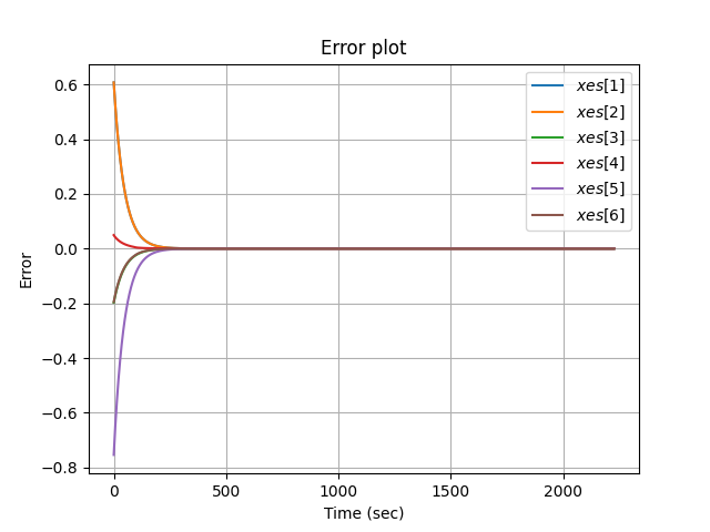
The best controller is the best, as it should be. It was chosen because it has no overshoot or oscillation. Although it is not particularly fast (as seen in the error plot), for this application, this slower, more robust controller is better than one that is fast with a lot of oscillation and overshoot.

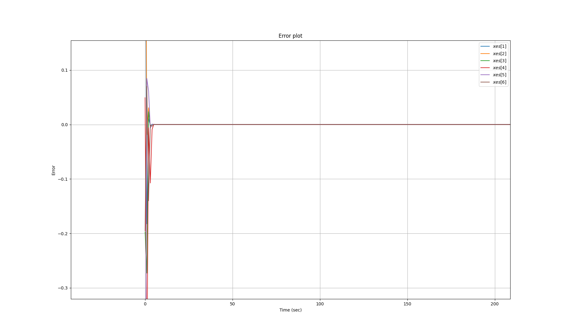
The overshoot controller, as seen in the figure below, has a lot of overshoot. Shocker. This is because it includes a large ki (= 60), which is often not used for robotics applications for this exact reason.


